Causes – Novel Ecosystems

Non-native species in the Anthropocene

Breaking dispersal barriers through human transport

Summary: Trade routes and the evolution of transportation technology have increased thefrequency and magnitude of non-native species invasions. The geographical isolation of species hasbeen eroded by human travel and climate change has been found to increase habitat availability fornon-native species. Invasions can have negative consequences for native species, ecosystemfunctioning, and the economy. In this essay, I discuss few examples in literature and suggestions ofhow ecological hypotheses could be addressed under the novel ecosystems framework, as itpertains to trade routes and movement of species. Understanding the effects of invasion mediatedthrough a global network of transport is important in order to further address how climate change,transport routes and species-specific traits will affect the native communities in which the invaders

will arrive.

Globalization is “the process in which people, ideas and goods spread throughout the world,

spurring more interaction and integration between the world’s cultures, governments and economies” (Globalization, n.d.). From an ecological perspective, the spread of goods and integration between economies also facilitates the release of non-native species, due to transport vectors and pathways increasing in number and frequency of use. Advances in navigation technology also mean that the speed and the scale of species movement will continue to increase (Figure 1).This creates an interesting phenomenon not only for biologists studying communities and their resilience, but also throws in a challenge for public policy and management of species.

Figure 1. a.) This figure depicts the general trend in increasing number of shipments and the number of specimens to the USA, from period 2000-2006 (R2 = 0.76). b.) Gross domestic product as a proxy for intensity of transport, the more a nation trades, the higher its GDP; the higher its GDP, the more non-native species a nation will harbor. This figure shows the relationship between gross domestic product and non-native plant richness for some islands and continental regions of the world. Continents R2 = 0.42, P < 0.01; Islands R2 = 0.54, P < 0.05.
Lockwood, Julie L., Hoopes, Martha F., and Marchetti, Michael P.. Invasion Ecology (2). Somerset, GB: Wiley-Blackwell, 2013.
(a) Adapted from Smith, K.F., Behrens, M., Schloegel, L.M., Marano, N., Burgiel, S. and Daszak, P. (2009) Reducing the risks of the wildlife trade. Science 324 , 594– 595.
(b) Adapted from Hulme, P.E. (2009) Trade, transport and trouble: managing invasive species pathways in an era of globalization. Journal of Applied Ecology 46 , 10– 18.

Non-native species have challenged expectations under various theoretical frameworks in population biology, population genetics, and ecology. One interesting aspect of non-natives and human transport is that we are removing barriers of dispersal for species. In island biogeography theory, distance to suitable habitat is a key predictor of species richness, however, in today’s world distance alone might not tell us much about the capacity of an area to carry certain number of species (Figure 2). When dispersal barriers are removed, researchers are looking to climate similarity and transport vectors to better predict the success of a species in colonizing a new area. Capinha and colleagues (2015) empirically tested how a break in biogeographic boundaries via human transport makes climate and trade relationships the best variables to explain species distributions.Thus suggesting that climate and perhaps socioeconomic relationships will define the new biogeography of the Anthropocene. Other researchers are also drawing the same conclusions, such as Helmus et. al. (2014) in their study about Anolis lizard diversity among Caribbean islands, who concluded that the amount of economic trade via shipping was a better predictor of species diversity than geographic isolation alone.

Figure 2. (a) The linearization of the Caribbean anole species–area relationship (SAR) and (b) the flattening of the species–isolation relationship (SIR) after considering transport pathways. In this figure, blue-colored lines represent expectation under classic island biogeography, whereas red-colored lines was the trend found by Helmus et. al. 2014. The number of species used to be dominated by colonization and speciation, respectively. However, when considering modern shipping, colonization became the major force on all islands.
Edited from: Helmus, M.R., Mahler, D.L., Losos, J.B. (2014). Island biogeography of the Antrhopocene. Nature, 513, 543-546

Erle Ellis, an advocate for the Anthropocene, lamented in an interview that ecologists are resistant to include human factors into ecological models (Singer 2014). Ambivalence continues around the idea of including human agency either as a component of novelty or as requirement for our studies on novelty going forth, perhaps since human influence is so prevalent. Humans have been reshaping the Earth since the Late Pleistocene, altering the landscape, domesticating certain species and even expanding species ranges, and so it seems daunting to account for human influence in models. However, we are living in a time where our own technological advances provide us with powerful tools to study how our societies drive climatic and biogeographic patterns. We can now get detailed information from current and past legacies (stable isotopes, ancient and mtDNA,remote sensing, etc.) in order to quantify the extent and intensity of anthropogenic alterations and its effects on biodiversity. As evidenced in a paper on anthropogenic shaping of global species distributions, Bovin et. al. 2016 used multiple molecular, computational and archeological evidence to show how human transformations have created novel ecosystems around the world. The changes in ecosystems and spread of non-native species were and still are primarily mediated by human migrations and their economies.

Non-native species transport and human agency are so intertwined that the way in which our economies work could dictate how many species – and at what rate- will assemble in a given area.This might mean that as more countries become active in the global trade network, inevitably the risk of introducing species will increase. Further, the number of trade routes and number of visits can increase propagule pressure (introduction effort, or the number of individuals introduced to into a region) which is a key element of invasive species persistence.

A great opportunity for research given this situation is the study of novelty from the biotic perspective. One example might be by contributing to the body of research under the biotic resistance hypothesis, which states that diverse biotic communities are more resistant to an invasion. This hypothesis was based on Sir Elton’s work on how the combination of predation,competition, and aggression can act as a barrier to invasive species establishment and abundance.Nevertheless, there is still a lack of understanding on the mechanisms underlying the variation in susceptibility of biotic communities to species invasion. Under the novel ecosystem framework, we might be able treat trade routes as a source of biotic novelty. As a first step, we can identify older trade routes versus newer ones, quantify the number of native and nonnative species present and compare the species richness, evenness and function in each region at different scales from a port. A significant difference in these numbers can allow us to test hypothesis about biotic resistance to invasion. Further, by looking at differences in species function between two regions differing in number of trade routes and usage, we might be able to assess how trade routes can also serve as an agent of biotic homogenization.

~by Diana Guzman Colon~

Boivin, N. L., Zeder, M. A., Fuller, D. Q., Crowther, A., Larson, G., Erlandson, J. M., … Petraglia, M. D.(2016). Ecological consequences of human niche construction: Examining long-termanthropogenic shaping of global species distributions. Proceedings of the National Academy ofSciences , 113(23), 6388–6396. http://doi.org/10.1073/pnas.1525200113

Capinha, C., Essl, F., Seebens, H., Moser, D., & Pereira, H. M. (2015). The dispersal of alien speciesredefines biogeography in the Anthropocene. Science, 348(6240), 1248–1251.http://doi.org/10.1126/science.aaa8913

Globalization. (n.d.). Retrieved December 13, 2016, from https://www.merriam-webster.com/dictionary/globalization

Helmus, M.R., Mahler, D.L., Losos, J.B. (2014). Island biogeography of the Antrhopocene. Nature,513, 543-546. http://doi.org/10.1038/nature13739

Singer, E. (2014, October). Lizard stowaways revise principle of Ecology. Scientific American. Retreived from http://www.scientificamercian.com/article/lizard-stowaways-revise-principle-of-ecology

Quantifying Novelty

Executive Abstract

Since its introduction, the term “ecological novelty” has generated quite a lot of controversy in the scientific community. In response to repeated cycles of critiques and responses among proponents and detractors, the definition has been tweaked again and again. Yet the term remains more or less binary; a certain place either is or is not novel. Such a definition requires an enormous amount of elaboration on the specific terms – novel relative to what? measured how? – in order for each application of novelty to be understood in context. And comparing novelty among different places is nearly impossible. Due in part to these limitations, scientists are considering alternative ways to define novelty on a spectrum. Such a continuous, quantitative approach would address much of the recent controversy, and open up avenues for new scientific understanding.

Preamble

With increasing attention focused on anthropogenic alterations to global ecosystems (e.g., “novel,” “no-analog,” or “emerging ecosystems”), moving beyond categorical classifications of novelty is useful. The original conception of novelty was binary; either a place was or was not novel. Many scientists feel that some of the controversy that has shadowed the term novelty since its introduction may have been avoided if the original authors had proposed a “spectrum” of novelty. Such a continuous spectrum would avoid difficult questions with the current definition of novelty. For example, since human activity has chemically modified the Earth’s atmosphere, could one argue that the entire Earth is then novel? And, if the whole planet is novel, is there any utility in labeling particular places or habitats as such?

Some of the advantages conferred by quantifying novelty in a continuous, rather than binary, way include:

1) prioritization of management or restoration goals
2) better accommodation of a non-binary and very complex world
3) partitioning variance in communities among multiple axes of abiotic and biotic change
4) communication and public outreach

However, quantifying novelty in a robust and meaningful way can be challenging.

Quantifying Abiotic Novelty

In some ways, because of the wealth of both historical and projected future data, quantifying novelty of climate or other abiotic factors is more tractable than quantifying biotic novelty. Williams and colleagues (2007) present an example of this by taking four climate parameters (summer and winter temperature and precipitation) from the Intergovernmental Panel on Climate Change projections from the year 2100. The authors quantify abiotic novelty as the dissimilarity (measured as the standardized Euclidean distance) in future climate space relative to present day conditions (Fig. 1). Because temperature and precipitation are important determinants of many ecological processes, shifts in climate such as those mapped in Figure 1 will likely impact biotic communities as well. In addition to the above quantitative assessment, the authors provide a conceptual figure (Fig. 2) demonstrating likely extinctions and novel species assemblages that may result from these projected future climates.

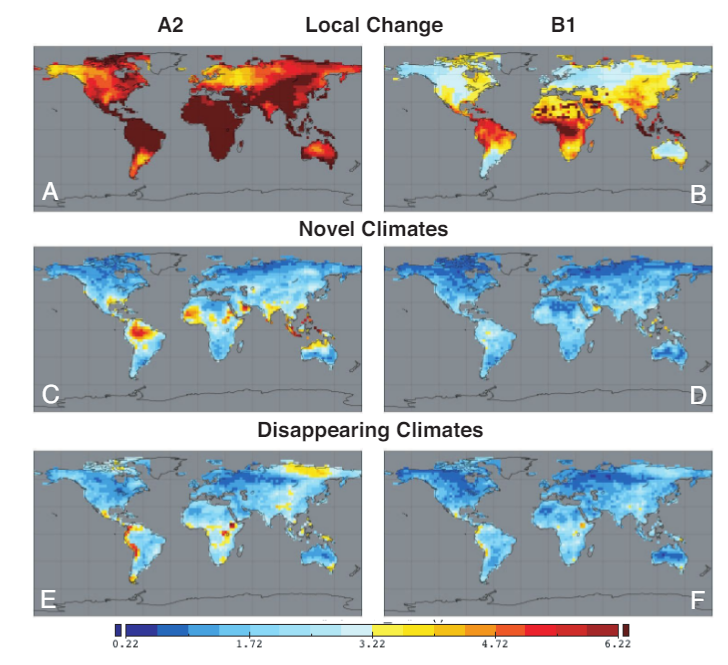
Figure 1 (from Williams et al. 2007, PNAS). Global maps of projected 2100 local climate change, arising novel climates, and disappearing climates based on the IPCC A1 (rapid; A, C, E) and B2 (mild, B, D, F) climate scenarios. Models were built using temperature and precipitation data from summer and winter months.

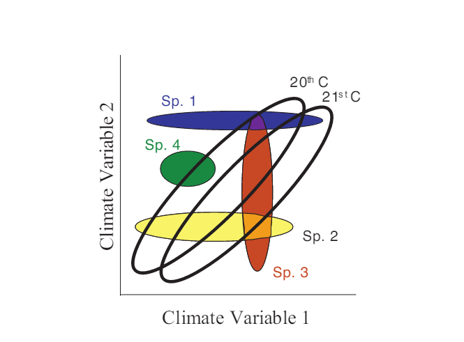
Figure 2 (from Williams et al. 2007, PNAS). Conceptual figure diagramming the fundamental niches of four species (colored ellipses) and potential future shifts under novel climate parameters.

Quantifying Biotic Novelty – Challenges

Quantifying biotic novelty presents an additional set of challenges and considerations, especially if the goal is to compare multiple measures of novelty across multiple communities. Historically, these comparisons have tended to be more descriptive than hypothesis driven (Weinstein et al. 2014), and are complicated by the fact that opposing responses to global changes at the species-level tend to render the corresponding community-level changes weak or undetectable (Supp and Ernest, 2014). Furthermore, comparisons of novelty (where novelty is quantified using dissimilarity in species composition as a proxy of novelty) across multiple study systems are also difficult because measures of beta diversity are sensitive to both sampling effort and regional species pool (Bennett and Gilbert 2015).

Another challenge for comparing biotic novelty among systems or regions is that many of the methods recently developed (e.g., Baselga 2010, 2012, Podani and Schmera 2011, Carvahlo et al 2012, Almeida-Neto et al 2013) employ multivariate methods originally designed for spatial comparisons among sites to describe temporal differences among communities. Temporal change has several unique properties (e.g., lack of physical boundaries, unidimensionality, autocorrelation, and directionality) that must be taken into account in analysis, making spatial measures of change a clumsy tool for time series data (Shimadzu et al 2015, Dornelas et al 2013).

Due to the challenges described in the above two paragraphs, comparisons of biotic novelty across space or time require carefully matching analytical methods to the question(s) and dataset(s) of interest. Relevant tools, methods, advice, considerations, etc. are described in the following paragraphs.

Quantifying Biotic Novelty – Some Best Practices

Much of the recent literature focused on quantifying differences between communities in space and time via alternative formulations of beta diversity is authored by Baselga (2010, 2012, 2013). His metric produces a multiple-site dissimilarity measure (can also be formulated to produce pair-wise dissimilarity, depending on data set) which separates beta diversity into two components: turnover (i.e., species replacement) and nestedness (i.e., species loss) (Fig. 3). Baselga argues that these two processes represent unique ecological phenomena, and disentangling their relative contributions can test interesting and relevant hypotheses that aren’t possible with traditional measures of beta diversity. This metric seems to have been widely adopted: the corresponding R package has been cited 62 times (as of 2016), while the 2010 paper that introduces his framework has been cited 267 times.

Figure 3 (from Baselga, 2010 Global Ecology and Biogeography). Conceptual figure demonstrating differences between turnover and nestedness. Both processes can contribute to biotic novelty.

Comparing changes in the novelty of the same community across time is best accomplished with measures of change that are explicitly formulated to describe temporal processes. Observations of temporal change can result from four different processes: measurement error, process error (i.e., significant drivers of change not considered in model), historical influence (i.e., autocorrelation—past community can influence contemporary community, but not vice versa), and systematic change (Dornelas et al. 2013). Shimadzu et al (2015) present a metric for comparing community change that accommodates these properties of temporal change. They break temporal turnover into two components – change in community composition and change in community size (aka capacity) – and from these components (with some fancy math) calculate a metric that, when tested with both real and simulated data, offers additional insights into temporal dynamics as compared with the borrowed spatial metrics. One such insight is the ability to identify any species AND any environmental factors which are important in driving the observed change.

A Very Simple Metric of Biotic Novelty

Perhaps the simplest metric for quantifying novelty is proposed by Helm et al (2015). They formulate a new index “Index of Favorable Conservation Status” which is calculated as the log ratio of characteristic:derived diversity, where characteristic diversity is that which should be there (i.e., native species in historical range) and derived diversity are those species which shouldn’t be there (i.e., non-native species or species not in historical range). Although this metric involves subjective decision making, there is value in this approach. It is simple and expert-based and therefore could be useful for managers and decision-makers, if not for ecologists. The authors suggest that this index captures conservation needs and adverse responses to global change in relative terms, and can be compared across regions and habitat types, can also be used to measure restoration success.

Closing Thoughts

There is plenty of room for development and advancement of analytical techniques that measure novelty. At current, we define ecological novelty much the same way Supreme Court Justice Potter Stewart described his threshold test for obscenity: “you know it when you see it.” Such qualitative assessments could be improved through the testing and development of rigorous quantitative techniques to describe and make inferences about novel ecosystems.

~by Amy Alstad~

Baselga, 2012. The relationship between species replacement, dissimilarity derived from nestedness, and nestedness. Global Ecology and Biogeography.

Baselga 2010. Partitioning the turnover and nestedness components of beta diversity. Global Ecology and Biogeography.

Bennett and Gilbert 2015. Contrasting beta diversity among regions: how do classical and multivariate approaches compare? Global Ecology and Biogeography.

Dornelas et al. 2013. Quantifying temporal change in biodiversity: challenges and opportunities. Proveedings of the Royal Society B.

Helm et al 2015, Characteristic and derived diversity: implementing the species pool concept to quantify conservation condition of habitats. Diversity and Distributions.

Shimadzu et al. 2015. Measuring temporal turnover in ecological communities. Methods in Ecology and Evolution.

Supp and Ernest. 2014. Species-level and community-level responses to disturbance. Ecology.

Weinstein et al. 2014. Taxonomic, phylogenetic, and trait beta diversity in South American Hummingbirds. The American Naturalist.

Williams, Jackson and Kutzbach. 2007. Projected distributions of novel and disappearing climates by 2100. Proceedings of the National Academy of Science.

Abiotic Novelty

Dams are ubiquitous and pervasive drivers of abiotic novelty; they create novel habitats for non-native species and can facilitate their spread.

Abstract

Human agency often results in increased abiotic novelty, which can facilitate theestablishment and spread of non-native species. I use dams as a case study to explore the causesand consequences of novelty in aquatic ecosystems from an invasive species perspective. Damsinteract with the invasion process in several ways. They fundamentally transform rivers to createmore ideal habitat for non-native species, both up and downstream. They also act as a steppingstone for invasive species to other nearby ecosystems.

Abiotic novelty can be a significant facilitator of non-native species. Often, increased abiotic novelty makes habitats more hospitable to non-native species, impacts native species, and in some cases, aids in spread of non-native species. Such abiotic novelty is often associated with human agency and comes in many forms. For example, strong abiotic drivers such as climate change allow for non-native species and native invaders to expand their ranges (Walther et al.2009), while land-use change can facilitate the invasion process via edge effects, reduced predation, or niche construction. The establishment of non-native species in freshwater aquatic systems altered by dams and canals is a particularly pervasive issue that illustrates both the causes and consequences of abiotic novelty following human agency.

Dams are ubiquitous on human dominated landscapes (Vörösmarty et al. 2010). They fundamentally transform upstream and downstream habitats, often to the detriment of native species and the benefit of non-native species. Primarily, dams and canals facilitate non-nativespecies in three ways. They create new habitats that are easier to exploit by non-native species.Dams also facilitate invasion in downstream habitats by altering the disturbance regimeassociated with high flow events. Additionally, dams and canals can facilitate the spread of non-natives. All in all, dams represent a systemic driver of abiotic novelty that facilitates non-native species.

Global relative dam density map showing how prevalent dams are. Vörösmarty et al. 2010. Supplemental material.

The new habitats created by dams and canals are easily invaded by species that are well adapted to lakes or lowland rivers with low flow rates. The reservoir created can result in novel mixtures of native and non-native species because these systems have characteristics of rivers and lakes – natives are often adapted to rivers and non-natives are often adapted to lakes (Vondracek et al. 1989). Some of the more common non-native fish species that thrive in reservoirs include largemouth bass (Micropterus salmoides), bluegill (Lepomis macrochirus),channel catfish (Ictalurus punctatus), threadfin shad (Dorosoma petense) and common carp (Cyprinus carpio, Rahel 2002). Researchers in California documented strong associations between many of the aforementioned species and aquatic systems modified by dams and canals (Marchetti et al. 2004). In some cases, these species could not persist or would be reduced in population size if it were not for the novel ecosystems created by dams and canals (Kanehl etal. 1997). Many of the above examples are from North America, but the same generalizations about non-natives being facilitated by habitats created by dams can be made about European (Clavero et al. 2013) and South American reservoirs (Daga et al. 2015).

Furthermore, dams create abiotic novelty by effectively altering the disturbance regime of rivers by attenuating extreme flow events (Bunn & Arthington 2002). This has the dual impact of making conditions ideal for non-natives and impacting native species that are adapted to such regimes. These extreme flow events are integral to maintaining native species communities in rivers and floodplains. This is the case because rivers are environmentally harsh, and for species to persist, they need to be adapted to extreme hydrologic events. For example, the persistence of non-native fish communities in regulated rivers seems to be limited by extreme flow events (Marchetti & Moyle 2001).These extreme events also interact with floodplains and riparian habitats. This makes these events essential to maintaining native riparian plant species dominance. The loss of disturbance events following dam construction has facilitated the establishment of tamarisk (Tamarix spp.) in the Grand Canyon (Stromberg et al. 2007) and Phylacanascens in Australian rivers (Taylor & Ganf 2005). By changing the intensity and duration of extreme hydrologic events, dams are facilitating non-native species existence in downstream habitats.

From Lytle & Poff 2004. http://www.cell.com/trends/ecology-evolution/pdf/S0169-5347(03)00316-1.pdf

Dams and canals can play a key role in facilitating the spread of non-native species either by acting as a source population or aiding there spread. Invaded reservoirs can act as invasion hubs on the landscape when people unintentionally move organisms to uninvaded systems. For instance, research done in Wisconsin suggests that reservoirs can act as a landscape driver of dispersal for a number of non-native species, especially to natural lakes (Johnson et al. 2008). In other words, regional abiotic novelty can impact local systems, even if they are relatively undisturbed. Reservoirs can also disperse organisms to downstream habitats, especially passive dispersers such as zooplankton and zebra mussels (Driessenia polymorpha, Havel et al. 2005).Exacerbating these trends, canals are often associated with dams, which hydrologically connect previously isolated systems. In some cases, this has transported non-native species to other basins, again, especially those with easily dispersed life histories (i.e. larval stage of fish, etc).For example, striped bass are widespread throughout California’s water infrastructure, but the population was established in the San Francisco-San Joaquin bay estuary in the late 1800’s and has since moved southward using the state’s water conveyance infrastructure (Moyle 2002). Another more extreme case of the consequences of increased hydrologic connectivity are the non-native species in the Laurentian Great Lakes. By some estimates, there are over 180 non-native species in the Great Lakes, many transported via man-made canals and locks or associated boat traffic (Ricciardi 2006).

Map of California’s water infrastructure highlights not only the prevalence of dams but also how hydrologically connected everything has become. https://californiawaterblog.com/2012/02/09/insights-for-california-water-policy-from-computer-modeling/

In conclusion, dams, as a special case of a pervasive driver of abiotic novelty, facilitate the establishment and spread of non-native species. The question we are left with is what can we do with these heavily altered systems? Can they be restored? There are already extensive and optimistic efforts to restore rivers and their biota by removing dams (O’Hanley 2011).

For example, several dams have been removed from the Elwha River watershed in Washington with promising results (East et al. 2015). The high flow disturbance regime has been restored,although the response of non-native species in the watershed to restoration is unknown. In someinstances, it seems as if these highly novel systems are restorable, but only when we have the social capital. The next question is how do we build social capital to allow us to tackle larger problems in conservation?

~by K. Martin Perales

Bunn, S.E., Arthington, A.H., 2002. Basic Principles and Ecological Consequences of AlteredFlow Regimes for Aquatic Biodiversity. Environmental Management 30: 492–507.Clavero, M., Hermoso, V., Aparicio, E., Godinho, F.N., 2013. Biodiversity in heavily modifiedwaterbodies: native and introduced fish in Iberian reservoirs. Freshwater Biology 58:1190–1201.

Daga, V.S., Skóra, F., Padial, A.A., Abilhoa, V., Gubiani, É.A., Vitule, J.R.S., 2015. Homogenization dynamics of the fish assemblages in Neotropical reservoirs: comparingthe roles of introduced species and their vectors. Hydrobiologia 746: 327–347.

East, A.E., Pess, G.R., Bountry, J.A., Magirl, C.S., Ritchie, A.C., Logan, J.B., Randle, T.J.,Mastin, M.C., Minear, J.T., Duda, J.J., Liermann, M.C., McHenry, M.L., Beechie, T.J.,Shafroth, P.B., 2015. Large-scale dam removal on the Elwha River, Washington, USA:River channel and floodplain geomorphic change. Geomorphology 228: 765–786.

Havel, J.E., Lee, C.E., Vander Zanden, J.M., 2005. Do reservoirs facilitate invasions into landscapes? BioScience 55: 518–525.

Johnson, P.T., Olden, J.D., Vander Zanden, M.J., 2008. Dam invaders: impoundments facilitatebiological invasions into freshwaters. Frontiers in Ecology and the Environment 6: 357–363.

Kanehl, P.D., Lyons, J., Nelson, J.E., 1997. Changes in the Habitat and Fish Community of theMilwaukee River, Wisconsin, Following Removal of the Woolen Mills Dam. North American Journal of Fisheries Management 17: 387–400.

Marchetti, M.P., Moyle, P.B., 2001. Effects of Flow Regime on Fish Assemblages in a Regulated California Stream. Ecological Applications 11: 530–539.

Marchetti, M.P., Light, T., Moyle, P.B., Viers, J.H., 2004. Fish invasions in California watersheds: testing hypotheses using landscape patterns. Ecological Applications 14:1507–1525.

Moyle PB 2002. Inland Fishes of California. Berkeley: University of California Press.O’Hanley, J.R., 2011. Open rivers: Barrier removal planning and the restoration of free-flowing rivers. Journal of Environmental Management 92: 3112–3120.

Rahel, F.J., 2002. Homogenization of Freshwater Faunas. Annual Review of Ecology and Systematics 33: 291–315.

Ricciardi, A., 2006. Patterns of invasion in the Laurentian Great Lakes in relation to changes in vector activity. Diversity and Distributions 12: 425–433.

Stromberg JC, S J Lite, R Marler, C Paradzick, PB Shafroth, D Shorrock, JM White, & MSWhite. 2007. Altered stream flow regimes and invasive plant species: the Tamarix case. Global Ecology and Biogeography 16: 381–393.

Taylor, B. & Ganf, G.G. (2005) Comparative ecology of two co-occurring floodplain plants: thenative Sporobolus mitchellii and the exotic Phyla canescens. Marine and Freshwater Research, 56: 431–440.

Vondracek, B., Baltz, D.M., Brown, L.R., Moyle, P.B., 1989. Spatial, seasonal and dieldistribution of fishes in a California reservoir dominated by native fishes. Fisheries

Research 7: 31–53.

Vörösmarty, C.J., McIntyre, P.B., Gessner, M.O., Dudgeon, D., Prusevich, A., Green, P.,Glidden, S., Bunn, S.E., Sullivan, C.A., Liermann, C.R., Davies, P.M., 2010.

Globalthreats to human water security and river biodiversity. Nature 467: 555–561.Walther, G.-R., Roques, A., Hulme, P.E., Sykes, M.T., Pyšek, P., Kühn, I., Zobel, M., Bacher, S., Botta-Dukát, Z., Bugmann, H., others, 2009. Alien species in a warmer world: risks and opportunities. Trends in ecology & evolution 24: 686–693.

Harvest

That humans are affecting ecosystems across local to planetary scales is news to relatively few people today. Anthropogenic climate change, alteration of nutrient cycles, and land conversion are widely cited drivers of contemporary ecosystem novelty. These factors have absolutely resulted in new configurations of biotic and abiotic interactions which have no historical analog. However, these human impacts are relatively modern. Human ecosystem impacts can certainly be traced back millennia using historical records of fire, but at such small human population sizes these impacts were rarely likely to result in widespread creation of novel ecosystems (Koch & Barnosky, 2006).

But before the invention of the internal combustion engine, the Haber-Bosch process, or even the plow, humans may have been unknowingly creating novel ecosystems as hunters on the landscape. While there is ongoing debate regarding the degree to which the Quaternary megafaunal extinctions of North and South America were the result of human harvest or rapid climate change, it appears that humans arrived on the scene shortly before two-thirds of the world’s largest animals (>44 kg) went extinct (Barnosky & Lindsey, 2010). The loss of megaherbivores has been suggested to have increased fire frequency and created novel species assemblages in North America (Gill et al. 2009), suggesting that harvest may have been the first human-induced driver of novelty.

It may not be hard to imagine that the loss of two-thirds of the world’s megafauna as resulting in novel species assemblages and ecosystem functions. But perhaps more interesting to consider is the way in which harvest may affect various dimensions of ecosystem novelty. In one dimension, when a species is harvested to extinction the result is a novel community assemblage: previous species richness minus one. But, what of harvest to historically low levels? One might argue that as long as a species persists in its historical habitat, the ecosystem is not necessarily novel. Alternatively, one could argue that it depends on the relative difference in current abundance relative to a baseline of previous abundance. Further yet, one could argue that unless there are measurable and/or qualitative changes in ecosystem function as a result of high levels of harvest-induced mortality, harvest has not resulted in novelty.

Let’s consider two examples of more modern harvest effects in order to discuss novelty. First, the harvest of passenger pigeons (Ectopistes migratorius), ultimately to extinction. Passenger pigeons have been estimated to have once numbered between 3 and 5 billion, winging their way across northeastern North America in column-shaped flocks measuring 1 km wide by up to 450 km long. Ellsworth and McComb (2003) estimated that 3 billion passenger pigeons would have consumed between 300,000 and 1,500,000 hectares red oak acorn production—per day. Further, they suggest that the sheer roosting of these birds on trees would have led to damaged and overturned trees, and where the trees did remain erect, the ground would have been covered with up to 50 cm of excrement at regular roosting sites. The authors argue that passenger pigeons may have been responsible to maintaining white oak forest dominance in North America, and that their extinction may have facilitated the spread of red oak forest northward. The regular damage and seed consumption of oaks caused by the pigeons, the authors argue, may have created a more fire-prone landscape that favored white oaks due to their increased fire-tolerance relative to red oaks. The harvest to extinction of passenger pigeons has resulted in reduced species richness across their range, an event that Aldo Leopold eulogized at the dedication of the monument to the passenger pigeon at Wyalusing State Park, Wisconsin in 1947: “We meet here to commemorate the death of a species. This monument symbolizes our sorrow. We grieve because no living man will see again the onrushing phalanx of victorious birds, sweeping a path for spring across the March skies, chasing the defeated winter from all the woods and prairies of Wisconsin. Men still live who, in their youth, remember pigeons; trees still live that, in their youth, were shaken by a living wind. But a few decades hence only the oldest oaks will remember, and at long last only the hills will know.”

Their loss means a novel species assemblage in northeastern North America. But, did the loss of such great numbers of pigeons result in novelty in other dimensions? It’s highly likely, but the data to show if the disturbance regime has been substantially altered or if there are other organisms that now predate upon acorns or cycle nutrients with the same or similar efficacy are yet lacking.

A second modern case study of harvest leading to novelty comes from the commercial harvesting of whales. Commercial whaling has been going on for over 1000 years, and it’s estimated that total biomass of whales has been reduced by up to 85% from the pre-whaling era (Roman et al., 2014). While no whale species has been harvested to extinction, their cumulative scarcity in the oceans has resulted in the identification of 4 mechanisms of ecosystem alteration that have been consequently reduced. First, at their pre-whaling abundances in the North Pacific, whales would have required an estimated 65% of all primary production to maintain such large populations. While the same amount of primary production required to support one blue whale could support 1,500 penguins, the combined biomass of the penguins would only by approximately 8% of the blue whale owing to vast differences in metabolic efficiency. Therefore, as a result of reduced whale populations, less carbon is stored in these ecosystems or transported to the ocean floor upon death (Roman et al. 2014). The loss of whales is also have thought to result in altered phenotypes among krill, a favorite food of baleen whales.

The second mechanism by which reduced whale populations have altered oceanic ecosystems is the loss of important food sources for killer whales. It is thought that relative depletion of whales as prey for killer whales led to greater predation on smaller mammals, like sea otters, creating cascading effects that ultimately reduced the abundance of kelp forests off the coasts of Alaska and British Columbia. Thirdly, whales often feed at great depths but require breathing at the ocean surface. This vertical movement facilitates the movement of critical nutrients like nitrogen and iron by two mechanisms: whales, having filled up on food at depths defecate nutrient-rich plumes in surface waters causing increased surface productivity; and also by the mere movement of water along the drag of their bodies across the nutrient-rich depths and nutrient-poor surface waters. Finally, in death whales transport immense amounts of nutrients to the ocean floor. In fact, a single 40-ton gray whale can deliver the equivalent of >2000 years of carbon flux to the ocean floor to the area on which the carcass lands. In the North Pacific, 60 species of animals are known only from whale carcasses. Together, the restoration of whales to historical numbers would result in the transport of equivalent amounts of carbon to the ocean floor as proposed iron enrichment climate mitigation strategies have proposed (Roman et al. 2014).

Although whales haven’t become extinct, their size and critical historical ecosystem roles indicates that even the reduction in total numbers has created massive alterations and created novel pathways by which ecosystems function today.

~by Aaron Koning~

Barnosky AD, Lindsey EL. 2010. Timing of Quaternary megafaunal extinction in South America in relation to human arrival and climate change. Quaternary International, 217:10-29.

Ellsworth JW, McComb, BC. 2003. Potential Effects of Passenger Pigeon Flocks on the Structure and Composition of Presettlement Forests of Eastern North America.Conservation Biology, 17(6): 1548-1558.

Gill JL, Williams JW, Jackson ST, Lininger KB, Robinson GS. 2009. Pleistocene megafaunal collapse, novel plant communities, and enhanced fire regimes in North America. Science, 326:1100-1103.

Koch PL, Barnosky, AD. 2006. Late Quaternary Extinctions: State of the Debate. Annu. Rev. Ecol. Evol. Syst. 2006. 37:215–50.

Roman J, Estes JA, Morissette, L, Smith, C, Costa D, McCarthy, J, Nation JB, Nicol S, Andrew Pershing A, Smetacek V. 2014. Whales as marine ecosystem engineers. Frontiers in Ecology and the Environment, 12(7): 377–385.